Return & Volatility of a Multi-Asset Portfolio
January 31, 2021 by Chris
 statistics
In previous posts we discussed about the expected return (mean value of a distribution) and the volatility (standard deviation) of an asset.
But, in investing, we rarely hold a portfolio of just one stock! Let's start with two stocks and observe what happens with return and volatility.
The first question is: OK, what percentage of the total investment amount shall we allocate to stock A and what to stock B?
If we allocate 100% to A and 0% to B or the other way around, then we get into the "one asset" portfolio. Let's assume that we set weight w_A=50% on asset A and w_B=50% on asset B.
In that case, we are asked to come up with the return (mean) and the volatility (standard deviation) of the portfolio.
Someone would blindly assume that the Return = (w_A * R_A) + (w_B * R_B) and Volatility = (w_A * std_A) + (w_B * std_B). Well, maths keep always surprising us, and that is the case here!
While indeed the return of the 2 asset portfolio is the average weighted returns,
the volatility is
This second (2) equation tells us that the standard deviation of a 2 asset distribution is equal to the square root of the variance of asset A multiplied by the squared weight of A plus the variance of asset B multiplied by the squared weight of B, plus twice the product of the standard deviation of A times the standard deviation of B times the weight of A times the weight of B times the correlation coefficient of A and B!
So far so good! But where exactly does the magic begin? Well, the correlation coefficient is not always a positive number :O
The correlation coefficient can take values between -1 and 1. -1 when the two assets are perfectly negatively correlated, which means that when the first asset goes up the other goes down at the same pace and same angle. 1 when both assets move to the same direction with the same pace and same angle (either positive or negative direction) and 0 when the assets are totally uncorrelated. Values between -1 and 1 indicate a more loose correlation, but show the trend.
Back to the equation (2). If we have a negative correlation of the assets, the total volatility is less than the average volatility, and if we have a positive correlation the total volatility is more that the average.
It becomes pretty obvious that by just combining two non correlated assets we can achieve volatility sometimes even smaller than the assets' individually. Who wouldn't want that!
Keep in mind that where is the covariance of the two variables.
Let's see an example...
Real example of a two asset portfolio
At first, let's set the ground work to be able to fetch some stock prices.
Package Installation
%pip install yahoofinancials
from yahoofinancials import YahooFinancials
import pandas as pd
import matplotlib
import matplotlib.pyplot as plt
import seaborn as sns
import dateutil.parser
import numpy as np
def retrieve_stock_data(ticker, start, end):
    json = YahooFinancials(ticker).get_historical_price_data(start, end, "daily")
    columns=["adjclose"]  # ["open","close","adjclose"]
    df = pd.DataFrame(columns=columns)
    for row in json[ticker]["prices"]:
        d = dateutil.parser.isoparse(row["formatted_date"])
        df.loc[d] = [row["adjclose"]] # [row["open"], row["close"], row["adjclose"]]
    df.index.name = "date"
    return df

def normal_rets(S):
    return S.pct_change().dropna()
We are now ready to fetch prices. I have picked Microsoft Corporation (MSFT) and Alpha Pro Tech, Ltd. (APT). Below we see how the price of the stocks unfolded throughout 2020!
msft_stock_prices = retrieve_stock_data("MSFT", "2020-01-01", "2021-01-01")
msft_rets = normal_rets(msft_stock_prices).dropna()
msft_rets.columns = ['returns']

apt_stock_prices = retrieve_stock_data("APT", "2020-01-01", "2021-01-01")
apt_rets = normal_rets(apt_stock_prices).dropna()
apt_rets.columns = ['returns']

f, (ax1, ax2) = plt.subplots(1, 2, sharex=True)
msft_stock_prices.plot(figsize=(14,7), ax=ax1)
apt_stock_prices.plot(figsize=(14,7), ax=ax2)
ax1.get_legend().remove()
ax2.get_legend().remove()
ax1.title.set_text('MSFT Price Chart')
ax2.title.set_text('APT Price Chart')
plt.show()
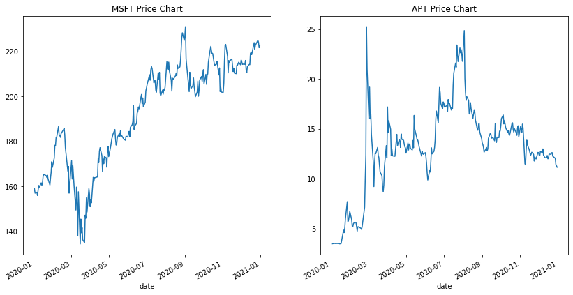
The graphs show some king of un-correlation. When one stock goes up the other goes down and vice versa. Let's explore the average return, standard deviation and correlation of the stocks.
msft_rets.mean().values[0], apt_rets.mean().values[0]
(0.0017171460669071206, 0.009654517798428635)
msft_rets.std().values[0], apt_rets.std().values[0]
(0.027679154652983044, 0.10987021868530256)
returns = msft_rets.merge(apt_rets, left_index=True, right_index=True)
returns.columns = ['MSFT', 'APT']
returns.corr()
| MSFT | APT | |
|---|---|---|
| MSFT | 1.0000 | -0.2182 |
| APT | -0.2182 | 1.0000 |
Obviously, both stocks yield a positive average daily return (small but positive), and while MSFT has a volatility around ~2.8%, APT is at ~11%, which denotes a very volatile asset. As expected, the correlation of the two assets is negative.
Let us now try to construct a portfolio of these two assets. From equations (1) and (2) we see that the weights are variable. We should also notice that the return is not a series of returns anymore but a single value. This value is the total return of an asset over the year. It is the so called Annualized Return.
def annualize_rets(r, periods_per_year):
    compounded_growth = (1+r).prod()
    n_periods = r.shape[0]
    return compounded_growth**(periods_per_year/n_periods)-1

annualized_returns = annualize_rets(returns, 252)
annualized_returns
MSFT    0.399429
APT     2.222543
dtype: float64
As you can see the annual return for 2020 for MSFT was ~40%, while for APT was ~220%! It is pretty obvious from the price graphs :)
Now, we move on and try to generate some portfolios where we assign different weights to the assets and try to calculate the return and the volatility of the portfolio. I will not get into what transposing a matrix means in algebra since it is not the focus of this post. Please check this wikipedia article for more info.
# from equation (1)
def portfolio_return(weights, returns):
    return weights.T @ returns

# from equation (2)
def portfolio_vol(weights, covariance_matrix):
    return (weights.T @ covariance_matrix @ weights)**0.5

# first we construct 10 pairs of weights like [(0.1,0.9), (0.2,0.8) ...]
weights = [np.array([w, 1-w]) for w in np.linspace(0, 1, 10)]

# then we calculate the return of the portfolio for each pair of weights
portfolio_returns = [portfolio_return(w, annualized_returns) for w in weights]

# and the volatility of the portfolio for each pair of weights
vols = [portfolio_vol(w, returns.cov()) for w in weights]

ef = pd.DataFrame({
    "Return": portfolio_returns,
    "Volatility": vols,
    "weights": weights
})

ax = ef.plot(x="Volatility", y="Return", style=".-", figsize=(11,6),
             title="2 Asset Portfolio Risk/Return", legend=False)
plt.ylabel("Return")

def label_point(x, y, val, ax):
  a = pd.concat({'x': x, 'y': y, 'val': val}, axis=1)
  for i, point in a.iterrows():
    prettified_p = f"({round(point['val'][0], 2)},{round(point['val'][1], 2)})"
    ax.text(point['x'], point['y'], prettified_p)

label_point(ef.Volatility, ef.Return, ef.weights, ax)

What the graph above tells us is that by combining the two assets we are able to achieve a total volatility (risk) that is less than each asset's individual volatility!
Observe the left most point on the graph!
In a next post we will calculate the optimal weights that minimize the risk of a portfolio as well as explore portfolios with more than 2 assets.
Some More Notes
- The approach I followed above is not something new. Is called Markowitz Model and won a Nobel Price in 1990.
- I tried to oversimplify the example, just to show the basics.
- I randomly picked the two assets, in the example, from IMPACTOPIA.
- We will prove, later on, that volatility changes over time :) and that would normally lead to rebalances.
- As always,
Historical returns are no guarantee of future returns.
Stay tuned ...

