Measures of Location

In investing, we are often presented with the challenge to analyze a data set (with historical prices of stocks, funds, etc.).

We are asked to answer questions like:

• What is the average return of a stock the last x days (given the daily returns)?
• What is the return of a stock that occurred the most the last x days?
• etc.

To answer, we commonly start by exploring some attributes that best describe the data. We often call them Measures of Location.

The most common measures of location are the Mean, Median and Mode.

Mean (or Average, or Expected Value) and Root Mean Square (RMS)

Mean is the sum of the values of the data points divided by the number of data points. That is,

But, what if we have a sequence like 0 4 1 -4 -1? The Mean will be 0! In that case we reside to the RMS which is

Median

Is the value of the point which has half the data smaller than that point and half the data larger than that point.

Mode

Is the value of the random sample that occurs with the greatest frequency (might not be unique).

Example

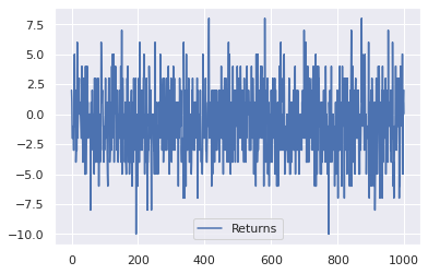
Let us generate some random data to showcase the above. We use random.normal here, which generates normally distributed numbers (we will discuss about normality in a following article) between -10 and 10. In terms of Investing, think of it as the simple returns (return = the percentage change of the today's closing price, over the yesterday's closing price) of a stock over a period.

import pandas as pd
import numpy as np
import matplotlib.pyplot as plt
import seaborn as sns
sns.set() 

randomInts = np.random.normal(loc=10, scale=3, size=1000).astype(int)-10

df = pd.DataFrame(randomInts, columns=['Returns'])
df.plot();

Mean

df.Returns.sum()/df.Returns.size

-0.612

# or
mean = df.Returns.mean()
mean

-0.612

Which is the answer to: What is the average return of a stock the last x days?

Median

np.sort(df.Returns.values)[int(df.Returns.size/2)]

-1

# or
median = np.percentile(df.Returns,50)
median

-1.0

Mode

sample_data = [1,2,3,4,3,5,3,6,3,7,8,9]
sample_data_df = pd.DataFrame(sample_data, columns=['Returns'])
sample_data_df.Returns.mode()[0]

3

It is apparent from the above that the number with the most frequent appearance is the number 3. That is because the numbers are discrete.

But, in a sequence of data that is continuous, the numbers can take any value in a range, which means decimal part (fractions). In cases like that it is difficult to find a single number that is present more often in the set. And that is normally the case in investing (the returns can take any value). Thus, we have to follow another approach and that is to separate the data into buckets. Here is where the notion of the histogram comes into play and generates an outcome like:

df.plot.hist(bins=50, figsize=(12,6), grid=True);

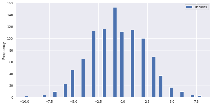
What really happens is to order the values in ascending order and then separate them in a number of buckets. For example if the min value is 1 and the max 10 and we split them in 9 buckets, the first one will include all numbers from 1 to 2, the second all numbers from 2 to 3 and so on. The next step is to find the bucket with the highest amount of elements and take the middle value.

counts, bins = np.histogram(df.Returns, bins=50)
max_index_col = np.argmax(counts, axis=0)
mode = bins[max_index_col]
mode

-1.0

# or
df.Returns.mode()[0]

-1

Alternative Measures of Location

In addition to the more common measures, there are several more that can also be included to the investing algorithms.

• Mid-Mean - computes a mean using the data between the 25th and 75th percentiles.
• Trimmed Mean - similar to the mid-mean except different percentile values are used. A common choice is to trim 5% of the points in both the lower and upper tails, i.e., calculate the mean for data between the 5th and 95th percentiles.
• Winsorized Mean - similar to the trimmed mean. However, instead of trimming the points, they are set to the lowest (or highest) value. For example, all data below the 5th percentile are set equal to the value of the 5th percentile and all data greater than the 95th percentile are set equal to the 95th percentile.
• Mid-range = (largest + smallest)/2.

Mid-Mean

# p_25 = df.Returns.quantile(0.25)  # Much slower than np.percentile
p_25 = np.percentile(df.Returns,25) # attention : the percentile is given in percent (5 = 5%)
p_75 = np.percentile(df.Returns,75)
mid_mean = df[df.Returns.gt(p_25) & df.Returns.lt(p_75)].Returns.mean()
mid_mean

-1.010498687664042

Trimmed-Mean

p_5 = np.percentile(df.Returns,5)
p_95 = np.percentile(df.Returns,95)
trimmed_mean = df[df.Returns.gt(p_5) & df.Returns.lt(p_95)].Returns.mean()
trimmed_mean

-0.5480427046263345

Winsorized Mean

data_indexes_to_stay_same = ( df.Returns > p_5 ) & ( df.Returns < p_95 )
data_to_stay_same = df[data_indexes_to_stay_same]
all_data_bellow_p_5 = df[df.Returns <= p_5].copy()
all_data_bellow_p_5.Returns.values[:] = p_5
all_data_above_p_95 = df[df.Returns >= p_95].copy()
all_data_above_p_95.Returns.values[:] = p_95
winsored_rets_list = [all_data_bellow_p_5, data_to_stay_same, all_data_above_p_95]
winsored_rets = pd.concat(winsored_rets_list)
winsored_mean = winsored_rets.Returns.mean()
winsored_mean

-0.608

Mid-range

mid_range = (df.Returns.max() + df.Returns.min())/2
mid_range

-1.0

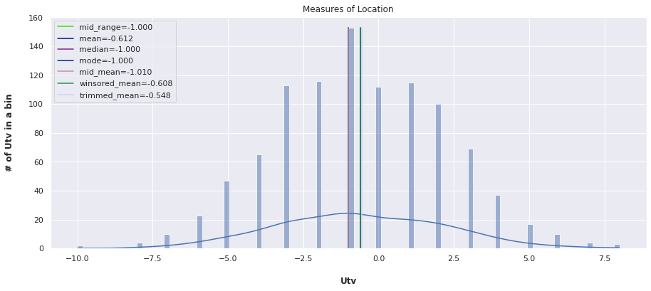
All Together

# df.Returns.plot.hist(bins=200, figsize=(15,6), grid=True)
plt.figure(figsize=(15,6))
sns.histplot(df.Returns, kde=True, bins=100)
plt.title("Measures of Location")
plt.xlabel("Utv", labelpad=20, weight='bold', size=12)
plt.ylabel("# of Utv in a bin", labelpad=20, weight='bold', size=12)
plt.axvline(x=mid_range, label='mid_range={:.3f}'.format(mid_range), ymax=0.95, c=np.random.rand(3,))
plt.axvline(x=mean, label='mean={:.3f}'.format(mean), ymax=0.95, c=np.random.rand(3,))
plt.axvline(x=median, label='median={:.3f}'.format(median), ymax=0.95, c=np.random.rand(3,))
plt.axvline(x=mode, label='mode={:.3f}'.format(mode), ymax=0.95, c=np.random.rand(3,))
plt.axvline(x=mid_mean, label='mid_mean={:.3f}'.format(mid_mean), ymax=0.95, c=np.random.rand(3,))
plt.axvline(x=winsored_mean, label='winsored_mean={:.3f}'.format(winsored_mean), ymax=0.95, c=np.random.rand(3,))
plt.axvline(x=trimmed_mean, label='trimmed_mean={:.3f}'.format(trimmed_mean), ymax=0.95, c=np.random.rand(3,))
plt.gca().legend(loc="upper left")
plt.show()