From Portfolio Wealth Index to Index Funds
February 5, 2021 by Chris
 python
Imagine a scenario where you have invested 100$ in a stock the last 3 years and you earned 20% in the 1st year, -10% in the 2nd year, and 11% in the 3rd year. You would like to see how the investment progressed over the time until today.
We have already discussed about geometric progression and the compounding of returns in a previous article, and we will use that knowledge even further here.
So, at the end of the 3rd year, the investment would be:
In the case of an initial investment of 1$, the result above would be called Cumulative Wealth Index!
Let me show you how this index progresses over time.
At first we set the ground work for fetching historical prices.
Package Installation
%pip install yahoofinancials
from yahoofinancials import YahooFinancials
import pandas as pd
import matplotlib
import matplotlib.pyplot as plt
import seaborn as sns
import dateutil.parser
import numpy as np
def retrieve_stock_data(ticker, start, end):
    json = YahooFinancials(ticker).get_historical_price_data(start, end, "daily")
    columns=["adjclose"]  # ["open","close","adjclose"]
    df = pd.DataFrame(columns=columns)
    for row in json[ticker]["prices"]:
        d = dateutil.parser.isoparse(row["formatted_date"])
        df.loc[d] = [row["adjclose"]] # [row["open"], row["close"], row["adjclose"]]
    df.index.name = "date"
    df.columns = [ticker]
    return df

def normal_rets(S):
    return S.pct_change().dropna()
Say, we have invested 100$ in the MSFT stock on the 11th of October 2019. Earlier we used annualized returns, but for this example we will use the daily returns.
Below we will download the stock prices for the aforementioned period and calculate the daily returns.
msft_stock_prices = retrieve_stock_data("MSFT", "2019-10-11", "2021-02-04")
msft_rets = normal_rets(msft_stock_prices).dropna()
msft_rets.head()
| MSFT | |
|---|---|
| date | |
| 2019-10-14 | -0.000931 |
| 2019-10-15 | 0.014475 |
| 2019-10-16 | -0.008194 |
| 2019-10-17 | -0.005128 |
| 2019-10-18 | -0.016322 |
Then, we will build the cumulative wealth index based on the initial investment, over time.
# See equation (1) in the post about geometric progression and the
# compounding of returns
wealth_index = 100 * (1 + msft_rets).cumprod()
wealth_index.head()
| MSFT | |
|---|---|
| date | |
| 2019-10-14 | 99.906939 |
| 2019-10-15 | 101.353104 |
| 2019-10-16 | 100.522643 |
| 2019-10-17 | 100.007156 |
| 2019-10-18 | 98.374868 |
And let's see how it looks like
f, (ax1, ax2) = plt.subplots(1, 2, sharex=True)
msft_stock_prices.plot(ax=ax1, figsize=(14,7))
wealth_index.plot(ax=ax2)
ax1.get_legend().remove()
ax2.get_legend().remove()
ax1.title.set_text('MSFT Price Chart')
ax2.title.set_text('Cumulative Wealth Index')
plt.show()
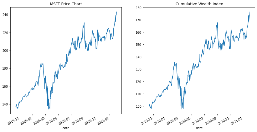
There are a few things to notice in the graphs above:
- The price development is the same :) and that makes sense, since the actual investment follows the price move of the stock.
- The start point is different. Since we invested only 100$ and not ~140$ (the price of one stock at the moment).
- The wealth index cares about the daily returns and not the actual price of the asset.
This last bullet allows us to extend the previous scenario by including more assets in our investment without taking into account the prices of the assets, but only the returns.
Portfolio Cumulative Wealth Index
I will simplify how a primitive index fund (or Mutual Fund or an ETF) is built by extending the process from the previous section.
Say now that, instead of investing 100$ to MSFT, we split the amount into 4 equal parts and we buy 4 different stocks. I will randomly pick Google's, Tesla's and Paypal's stocks.
from functools import reduce
google_stock_prices = retrieve_stock_data("GOOGL", "2019-10-11", "2021-02-04")
google_rets = normal_rets(google_stock_prices).dropna()

tsla_stock_prices = retrieve_stock_data("TSLA", "2019-10-11", "2021-02-04")
tsla_rets = normal_rets(tsla_stock_prices).dropna()

paypal_stock_prices = retrieve_stock_data("PYPL", "2019-10-11", "2021-02-04")
paypal_rets = normal_rets(paypal_stock_prices).dropna()

# bring them all together in a single dataframe
assets_returns = reduce(lambda left,right: left.merge(right, left_index=True, right_index=True),
            [msft_rets, google_rets, tsla_rets, paypal_rets])
assets_returns.head()
| MSFT | GOOGL | TSLA | PYPL | |
|---|---|---|---|---|
| date | ||||
| 2019-10-14 | -0.000931 | 0.001695 | 0.036589 | 0.001674 |
| 2019-10-15 | 0.014475 | 0.020094 | 0.003619 | 0.018084 |
| 2019-10-16 | -0.008194 | 0.000612 | 0.007212 | -0.004827 |
| 2019-10-17 | -0.005128 | 0.007884 | 0.008547 | 0.005238 |
| 2019-10-18 | -0.016322 | -0.006697 | -0.019163 | -0.023256 |
Based on the weight allocation of [.25, .25, .25, .25], let us now find the new cumulative wealth index of the investment.
# since the weights stay same throughout the index and since 100*0.25 = 25
portfolio_wealth_index = 25 * (1 + assets_returns).cumprod()
portfolio_wealth_index.head()
| MSFT | GOOGL | TSLA | PYPL | |
|---|---|---|---|---|
| date | ||||
| 2019-10-14 | 24.976735 | 25.042363 | 25.914720 | 25.041838 |
| 2019-10-15 | 25.338276 | 25.545567 | 26.008512 | 25.494683 |
| 2019-10-16 | 25.130661 | 25.561196 | 26.196096 | 25.371627 |
| 2019-10-17 | 25.001789 | 25.762725 | 26.419986 | 25.504527 |
| 2019-10-18 | 24.593717 | 25.590192 | 25.913712 | 24.911400 |
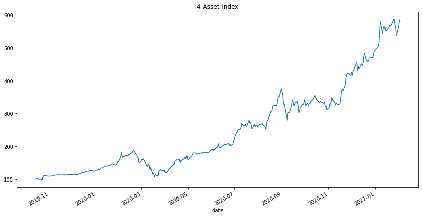
Now, we just fave to sum the columns per row and plot the result
portfolio_wealth_index.sum(axis=1).plot.line(figsize=(14,7))
plt.title('4 Asset Index')
plt.show()
Index/Mutual/Exchange-Traded Funds
In the example above, I chose some random assets and equally weighted them in a portfolio! However, even simplistic, this is how a traded fund looks like.
In practice, a fund is a bucket of assets weighted in a structured way, and initialized with a price (like i did above with the 100$). Then, they are offered in the stock exchange for purchasing. In our example above, if it was a traded fund, the investors would deposit money to the fund and the fund would buy the underlying assets based on the specified weights. The buying and selling of the fund, doesn't affect the price of the fund directly (but indirectly through the underlying assets).
The difference among the different types of funds is due to the way weights are calculated. Mutual and ETFs have managers that pick these weights based on market research, and other characteristics. The managers, can change the weights by performing a rebalancing of the portfolio.
In index funds (also known as passive ETFs) the weights are usually based on market cap and maybe other attributes and require minimum intervention from a manager (and due to that are normally much cheaper than the other types of funds). In the simplest case, an index fund could follow all the assets of a specific industry and allocate the weights according to the market capitalization of each asset (divided by the total market cap of all the assets in the index) or just follow the same weighting strategy of a well known index, such as S&P 500.
In future posts, I will try to build (and invent) different types of funds.
Until next time!

