Higher Moments of a Distribution

We have already discussed about the mean and the variance of a series of data.

Mean is also called the 1st moment and variance the 2nd moment. The type to get a moment (the movement) about a non-random value c, of a density function is:

Before explaining the moments, we should first understand what a density function is. Commonly called probability density function (PDF).

Density Function

30 people are gathered in a house party. Let us measure their weights:

import pandas as pd
m_v = [56.8, 81.3, 47.9, 32.5, 24.1, 25.3, 14.3, 29.4, 71.3, 86.0, 54.2, 15.2,
       54.7, 25.1, 49.5, 1.9, 70.0, 69.6, 75.4, 38.9, 49.2, 22.5, 68.6, 60.1,
       52.7, 109.7, 38.9, 45.9, 47.7, 52.9]
values = pd.Series(m_v)
values.describe()

count     30.000000
mean      49.053333
std       24.001634
min        1.900000
25%       30.175000
50%       49.350000
75%       66.475000
max      109.700000
dtype: float64

What if we change the way we present the data, and instead of having them in a simple series, we try to split them up into buckets.

We will get the, so called, histogram of the values. It shows how the probabilities of measurement are distributed.

import matplotlib.pyplot as plt
histogram = values.plot.hist(bins=10, figsize=(10,5))
plt.show()

If we ask the question: What is the probability, the next person that joins the party, weights between 80 and 90 kilos?

To answer this question, we need to imagine as if the upper boundaries of the blue colored space above, are a continuous line, a curve. This curve is what we call PDF or density function.

from scipy.stats import norm
import numpy as np
x = np.linspace(min(values), max(values))
ax = values.plot(kind='hist', bins=10, figsize=(10,5), density=True)
pdf_fitted = norm.pdf(x, *norm.fit(values))
pd.Series(pdf_fitted, x).plot(ax=ax)
plt.show()

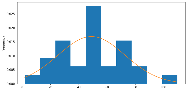
We observe that the curve is not a perfect fit. It is an approximation and there are hundreds of different curves we can plot and several of them will be very close to fitting the data (I will show that in another post).

In this case above, I have intentionally picked the data as such to resemble the, so called, normal distribution.

Back to our question now! The probability, the next person that joins the party, weights between 80 and 90 kilos, can be estimated by measuring the area below the curve for that bucket. So, if the whole area below the curve is 1 (zero moment, see below), the part that belongs to bucket 80-90 is a percentage :) and that is the probability we are after. The expression is:

Which is translated to: The probability a person weights between 80 and 90 kilos given an average of x and standard-deviation of y.

And the area below the curve is the integral between the points:

There are many pros in trying to use distributions to represent how the values in a dataset are distributed:

• makes it easy to measure the areas below (with integrals, since the function of the curve is known)
• the presentation is much better for the human
• well known distributions have really nice properties

Zero Moment (Total Mass)

That means that in (1), k=0 and as such $(...)^0 = 1$. That leaves us with:

Probability Distributions are normalized quantities, that always sum to one. Think of that as the probability that at least one of the events in a sample space will occur. Isn't that 100%?

1st Moment - Mean

c=0 in this case since we do not have an origin to get the moment (movement) about.

From (3) is obvious that we talk about the mean and that alternatively talk about the balance of the total mass (the area below the curve) around a point :)

2nd Moment - Variance

From (1), we can take c=0 and k=2! But what will that show us? How the mass is balanced around again the same point, which in practice is the average again but squared? Doesn't provide much value in understanding our data.

For that reason we get $c=μ$ and that will start making sense, since we se how the mass is diverging from the mean. It will show the variance of the data around the mean :)

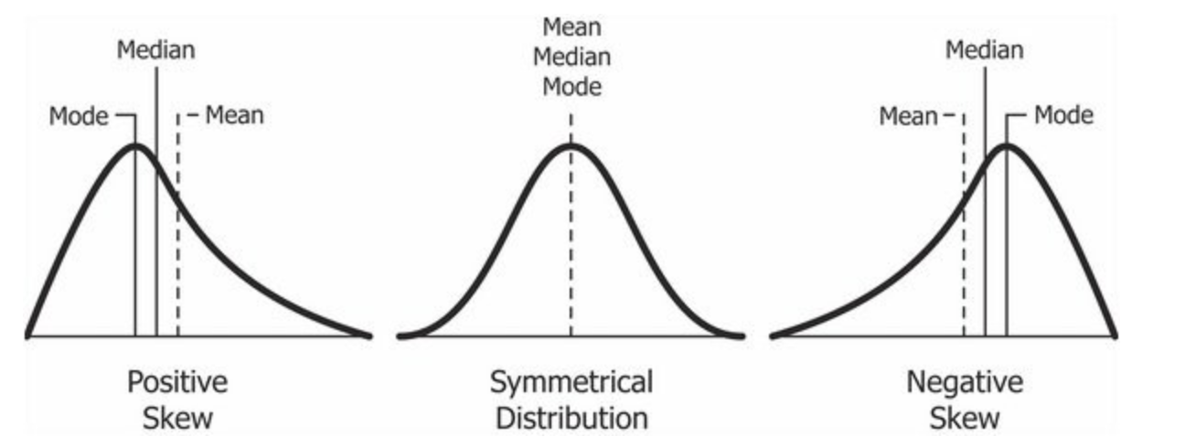
3rd Moment - Skewness

Following the pattern above and using k=3 around the mean $c=μ$ then we get the skewness which measures the relative size of the two tails of a distribution.

from scipy.stats import skew
skew(values, bias=False) # bias=False calculates the skewness and kurtosis of the sample as opposed to the population.

0.274192939649461

A left-skewed (negatively-skewed) distribution has a long left tail. That’s because there is a long tail in the negative direction on the number line. The mean is also to the left of the peak.

A right-skewed (positive-skew) distribution has a long right tail. That’s because there is a long tail in the positive direction on the number line. The mean is also to the right of the peak.

4th Moment - Kurtosis

The fourth central moment is a measure of the heaviness of the tail of the distribution.

from scipy.stats import kurtosis
kurtosis(values, bias=False)

0.14330737818315065

Higher Moments of the Normal Distribution

data = np.random.normal(0, 1, 10000000)
plt.hist(data, bins='auto')

print("mean : ", np.mean(data))
print("var  : ", np.var(data))
print("skew : ", skew(data, bias=False))
print("kurt : ", kurtosis(data, bias=False, fisher=False))

mean :  -0.00015674618345404924
var  :  1.0002202373014222
skew :  0.0007495220785926886
kurt :  3.0013415645199695

For a normal distribution the skewness is zero and the kurtosis is 3. These properties are specific to the normal distribution and are used for normality testing of distributions. We will go deeper in that in a later post.