Are Stock Returns Normally Distributed?

In a previous post we talked about the Higher Moments of a Distribution. We saw that skewness and kurtosis are two attributes that can identify if a distribution is normal or not (skewnes = 0 & kurtosis = 3).

Let's try this approach on the MSFT stock.

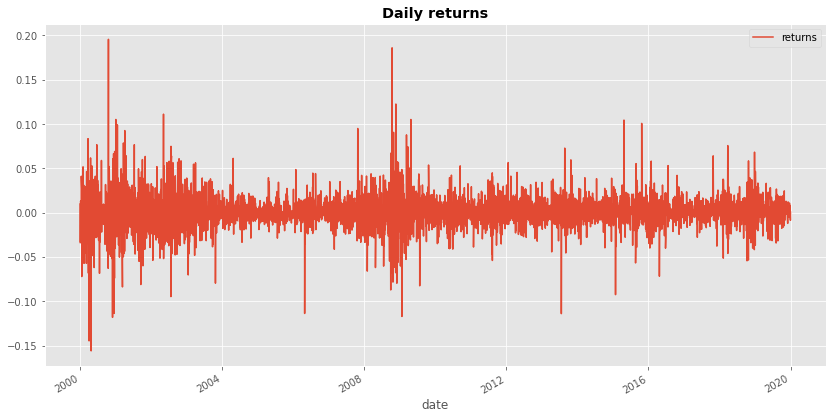
First step is to to fetch the data and print the returns.

%pip install yahoofinancials
from yahoofinancials import YahooFinancials
import pandas as pd
import matplotlib
import matplotlib.pyplot as plt
import seaborn as sns
import dateutil.parser
import numpy as np

matplotlib.rcParams['figure.figsize'] = (10.0, 5.0)
matplotlib.style.use('ggplot')

def retrieve_stock_data(ticker, start, end):
    json = YahooFinancials(ticker).get_historical_price_data(start, end, "daily")
    columns=["adjclose"]  # ["open","close","adjclose"]
    df = pd.DataFrame(columns=columns)
    for row in json[ticker]["prices"]:
        d = dateutil.parser.isoparse(row["formatted_date"])
        df.loc[d] = [row["adjclose"]] # [row["open"], row["close"], row["adjclose"]]
    df.index.name = "date"
    return df

def normal_rets(S):
    return S.pct_change().dropna()

def log_rets(S):
    rets = np.log(S) - np.log( S.shift(1))
    return rets[1:]

stock_prices = retrieve_stock_data("MSFT", "2000-01-01", "2020-01-01")

rets = normal_rets(stock_prices).dropna()
rets.columns = ['returns']
rets.plot(figsize=(14,7))
plt.title("Daily returns", weight="bold");

Let's find skewness and kurtosis:

from scipy.stats import kurtosis, skew
skew(rets, bias=False)[0], kurtosis(rets, bias=False, fisher=False)[0]

(0.20887713542026032, 13.229622042763442)

It is obvious that the MSFT stock returns (for that period) do not comply with the kurtosis and skewness of a normal distribution. Same, of course, happens if we get the log returns instead.

log_msft_rets = log_rets(stock_prices).dropna()
skew(log_msft_rets, bias=False)[0], kurtosis(log_msft_rets, bias=False, fisher=False)[0]

(-0.12981025399984283, 12.81366131030108)

Normality Tests

There are several interrelated approaches to determining normality:

• Histogram with the normal curve superimposed. Unfortunately, there is no automated way to represent the "fitness" as a value. This approach is empirical mostly and requires experience.
• Skewness & Kurtosis Tests.
• Normality plots. “Normal Q-Q Plot” provides a graphical way to determine the level of normality.
• Normality tests. The Kolmogorov-Smirnov test (K-S) and Shapiro-Wilk (S-W) test are designed to test normality by comparing your data to a normal distribution with the same mean and standard deviation of your sample. If the test is NOT significant, then the data are normal, so any value above .05 indicates normality. If the test is significant (less than .05), then the data are non-normal.

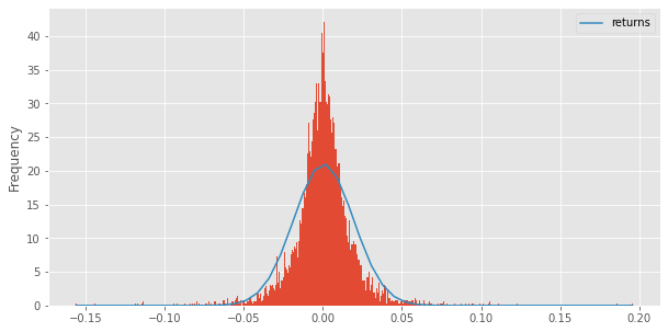
Histogram & Normal PDF

from scipy.stats import norm
x = np.linspace(min(rets.returns.values), max(rets.returns.values))
ax = rets.plot(kind='hist', bins=500, density=True)
pdf_fitted = norm.pdf(x, *norm.fit(rets.returns.values))
pd.Series(pdf_fitted, x).plot(ax=ax)
plt.show()

Skewness & Kurtosis Tests

from scipy import stats
stats.kurtosistest(rets.returns)

KurtosistestResult(statistic=29.93227785492693, pvalue=7.484189304773088e-197)

stats.skewtest(rets.returns)

SkewtestResult(statistic=5.99114785753993, pvalue=2.083650895527666e-09)

QQ-Plot

from numpy.random import seed
from statsmodels.graphics.gofplots import qqplot
from matplotlib import pyplot
seed(1)
qqplot(rets.returns, line='s')
pyplot.show()

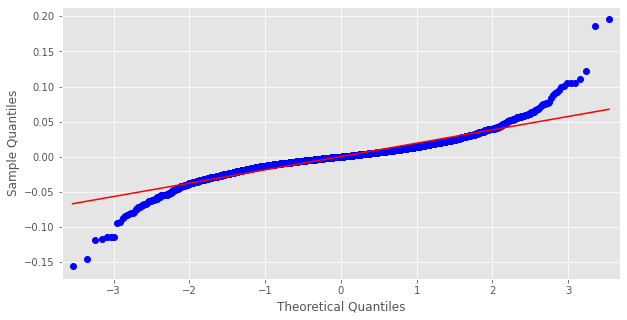
The Quantile-Quantile plot, as the name suggests, will compare the quantiles between the normal distribution and our data. We notice here that, the tails of the distribution of our data are diverging a lot from the normal distribution. This is what we would expect. Fat tails (leptokurtic)!

Statistical Normality Tests

The tests assume that the sample was drawn from a Gaussian distribution. Technically this is called the null hypothesis, or H0. A threshold level is chosen called alpha, typically 5% (or 0.05), that is used to interpret the p-value.

In the SciPy implementation of these tests, you can interpret the p value as follows.

• p <= alpha: reject H0, not normal.
• p > alpha: fail to reject H0, normal.

This means that, in general, we are seeking results with a larger p-value to confirm that our sample was likely drawn from a Gaussian distribution.

A result above 5% does not mean that the null hypothesis is true. It means that it is very likely true given available evidence. The p-value is not the probability of the data fitting a Gaussian distribution; it can be thought of as a value that helps us interpret the statistical test.

Kolmogorov-Smirnov test (K-S)

kstest = stats.kstest(rets.returns, 'norm')
kstest.pvalue > 0.05

False

Shapiro-Wilk Test

shapiro_stat, shapiro_p = stats.shapiro(rets.returns)
shapiro_p > 0.05

False

D’Agostino’s K^2 Test

The D’Agostino’s K^2 test calculates summary statistics from the data, namely kurtosis and skewness, to determine if the data distribution departs from the normal distribution. (named for Ralph D’Agostino)

• Skew is a quantification of how much a distribution is pushed left or right, a measure of asymmetry in the distribution.
• Kurtosis quantifies how much of the distribution is in the tail.

It is a simple and commonly used statistical test for normality.

seed(1)
dagostino_stat, dagostino_p = stats.normaltest(rets.returns)
dagostino_p > 0.05

False

Jarque-Bera Test for Normality

jarque_bera_stat, jarque_bera_p = stats.jarque_bera(rets.returns)
jarque_bera_p > 0.05

False

Conclusion

In this article we went through some techniques that allow us identify if stock returns are normally distributed. We saw, with examples, that returns (arithmetic, or log) are not normally distributed but instead exhibit fat tails. We cannot generalize, of course, just by looking into one stock, but I will leave that as a small exercise to the curious readers.

The question is still... Since the returns are not following a normal distribution, then what type of distribution do they follow?

The answer to that in Fit Multiple Distributions to Asset Returns!