Drawdown

In a previous post we talked about the wealth index of an asset as well as a portfolio of assets. The idea of the wealth index is very powerful because it represents the cumulative profit of an asset (since it depends on the price returns).

Now, if we have invested 100$ on an asset and we were asked to find the maximum loss, when did that happen and for how long did it last? We need to walk through our wealth index and find all the deeps, then see which one was the largest, when it did happen and when it finally recovered to the previous peak value.

We employ a well known measure of risk in Investing, called Drawdown.

Computation and Plotting of the Drawdown

First the ground code that allows us to fetch stock historical data.

%pip install yahoofinancials
from yahoofinancials import YahooFinancials
import pandas as pd
import matplotlib
import matplotlib.pyplot as plt
import seaborn as sns
import dateutil.parser
import numpy as np

def retrieve_stock_data(ticker, start, end):
    json = YahooFinancials(ticker).get_historical_price_data(start, end, "daily")
    columns=["adjclose"]  # ["open","close","adjclose"]
    df = pd.DataFrame(columns=columns)
    for row in json[ticker]["prices"]:
        d = dateutil.parser.isoparse(row["formatted_date"])
        df.loc[d] = [row["adjclose"]] # [row["open"], row["close"], row["adjclose"]]
    df.index.name = "date"
    df.columns = [ticker]
    return df

def normal_rets(S):
    return S.pct_change().dropna()

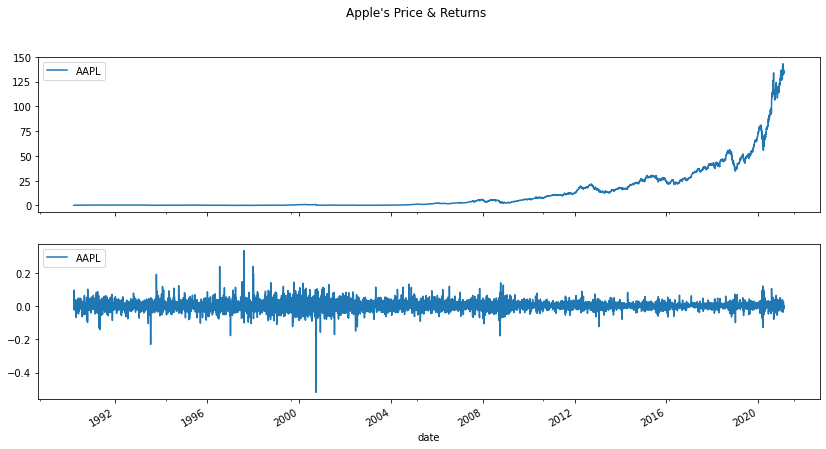
I'll randomly pick Apple's (AAPL) stock for this analysis.

apple_stock_prices = retrieve_stock_data("AAPL", "1990-03-14", "2021-02-17")
apple_rets = normal_rets(apple_stock_prices).dropna()
fig, (ax1, ax2) = plt.subplots(2, sharex=True, figsize=(14,7))
fig.suptitle("Apple's Price & Returns")
apple_stock_prices.plot(ax=ax1, label='Price')
apple_rets.plot(ax=ax2, label='Returns')
plt.legend(loc="upper left")
plt.show()

Say now that we invested 100$ late 2016. Let's build the wealth index like we did in this post, and find the peaks of the wealth index. That is, the highest generated wealth prices before a deep.

wealth_index = 100*(1+apple_rets.AAPL["12-2016":]).cumprod()
peaks = wealth_index.cummax()
ax = wealth_index.plot(figsize=(14,7), label="W-Index")
peaks.plot(ax=ax, label="Peaks")
plt.legend(loc="upper left")
plt.show()

Do you see these nice lagoons? Well, we wouldn't want them to be deep and long in duration, cause that is when our investment looses value and we have to wait until it recovers!

So, moving forward we want to find which lagoon was the deepest, how deep? and how long did it take to move back to the previous peak.

First things first, we have to measure at any given point what is the difference between the peak and the wealth index. For example, the peak at a given point is 220$ and the index is 150$. That means that the index is 70$ below the peak. Since our target point is 220$ and we have lost 70$, we can say that we we are $-\frac{70}{220}=31.8$% below the target.

drawdown =  (wealth_index - peaks)/peaks
drawdown.plot(figsize=(14,7), title="Drawdown")

The diagram above is what we call a Drawdown of an asset and it doesn't really have to do with any initial investment. Drawdown is a very nice indicator of risk since it is more realistic when compared to other risk indicators that involve standard deviations (Since returns deviate from normality as we proved in Are Stock Returns Normally Distributed)

Useful insights from the Drawdown

We are now ready to find the largest drawdown and the date that occurred.

drawdown.min(), drawdown.idxmin()

(-0.38515910000506054, Timestamp('2019-01-03 00:00:00'))

We see that on the 3rd of January 2019 our investment was loosing 38.5% of its value!

One step further, we will try to find how long the lagoons lasted and find the longest one and an average of their durations.

def compute_drawdown_lagoons_durations(drawdown):
  # find all the locations where the drawdown == 0
  zero_locations = np.unique(np.r_[(drawdown == 0).values.nonzero()[0], len(drawdown) - 1])
  # also assign the dates so we know when things were not sinking
  zero_locations_series = pd.Series(zero_locations, index=drawdown.index[zero_locations])
  # do a shift to show what is the last and previous non zero dates
  df = zero_locations_series.to_frame('zero_loc')
  df['prev_zloc'] = zero_locations_series.shift()
  # keep only the dates where the difference is more than 1
  # that denotes the lagoons
  df = df[df['zero_loc'] - df['prev_zloc'] > 1].astype(int)
  df['duration'] = df['zero_loc'].map(drawdown.index.__getitem__) - df['prev_zloc'].map(drawdown.index.__getitem__)
  df = df.reindex(drawdown.index)
  df = df.dropna()
  return df['duration']

df = compute_drawdown_lagoons_durations(drawdown)
df

date
2016-12-06     4 days
2016-12-13     4 days
2016-12-27     6 days
2017-01-06    10 days
2017-01-17     6 days
               ...   
2020-08-26     2 days
2020-08-31     5 days
2020-12-28   118 days
2021-01-21    24 days
2021-02-16    21 days
Name: duration, Length: 69, dtype: timedelta64[ns]

The DataFrame above prints the last day of a drawdown, and its duration in days.

df.max(), df.mean()

(Timedelta('372 days 00:00:00'), Timedelta('20 days 02:46:57.391304347'))

The longest drawdown lasted 372 days! and the average duration of a drawdown was 20 days :)

Stay tuned!