Fit Multiple Distributions to Asset Returns!
March 28, 2021 by Chris
 python
Earlier in Are Stock Returns Normally Distributed? we went through different ways to validate when asset returns are normally distributed. While we used only one stock to prove that stock returns are not normally distributed, the phenomenon applies to any volatile asset, in general.
The question though is: Really, which distribution do returns follow?
Below we load the MSFT stock returns as we did before!
Package Installation
%%capture
%pip install yahoofinancials
from yahoofinancials import YahooFinancials
import pandas as pd
import matplotlib
import matplotlib.pyplot as plt
import seaborn as sns
import dateutil.parser
def retrieve_stock_data(ticker, start, end):
    json = YahooFinancials(ticker).get_historical_price_data(start, end, "daily")
    columns=["adjclose"]  # ["open","close","adjclose"]
    df = pd.DataFrame(columns=columns)
    for row in json[ticker]["prices"]:
        d = dateutil.parser.isoparse(row["formatted_date"])
        df.loc[d] = [row["adjclose"]] # [row["open"], row["close"], row["adjclose"]]
    df.index.name = "date"
    return df

def normal_rets(S):
    return S.pct_change().dropna()

stock_prices = retrieve_stock_data("MSFT", "2019-01-01", "2020-01-01")

rets = normal_rets(stock_prices).dropna()
rets.columns = ['returns']
Fit all known distributions
Instead of trying to fit the Gaussian Distribution to our data, we will try to fit all the known (scipy.stats implementations) distributions and see which one (or ones) fits the data best.
import numpy as np
from scipy.stats._continuous_distns import _distn_names
import scipy.stats as st
import warnings

def fit_all_distributions(data):
    """
    Returns: Dict of the density function and the Sum of Squared Errors (SSE)
    """
    # Get histogram of original data. First, get the x for the pdf
    # second, get y to calculate the distance between the
    # distribution and the real data
    y, x = np.histogram(data, bins='auto', density=True)
    x = (x + np.roll(x, -1))[:-1] / 2.0

    dist_fit = {}

    # Estimate distribution parameters from data
    for distname in _distn_names:
        distribution = getattr(st, distname)

        # Try to fit the distribution
        try:
            # Ignore warnings for data that can't be fit
            with warnings.catch_warnings():
                warnings.filterwarnings('ignore')

                # fit dist to data
                params = distribution.fit(data)

                # Calculate fitted PDF and error
                pdf = distribution.pdf(x, *params)
                sse = np.sum(np.power(y - pdf, 2.0))
                dist_fit[distname] = {}
                dist_fit[distname]['pdf'] = pdf
                dist_fit[distname]['sse'] = sse
        except Exception:
            pass

    return dist_fit
dist_fit = fit_all_distributions(rets.returns)
len(dist_fit)
99
What? 99? :) Well, It should not be of a surprise that several distributions would fit the data. But the "fit" could be really off :) For example an exponential or even a uniform distribution could fit the data, but the squared error (the distance between the actual data points and the respective distribution points) would be really large compared to distributions that approximate the histogram of our data.
Let's get the 15 distributions with the lowest SSE (the ones that best fit the data).
dname_list = []
sse_list = []
pdf = []
for dname in dist_fit:
  dname_list.append(dname)
  sse_list.append(dist_fit[dname]['sse'])
  pdf.append(dist_fit[dname]['pdf'])

df = pd.DataFrame({'dist': dname_list, 'sse': sse_list, 'pdf':pdf})
df = df.sort_values('sse')
df_15 = df[:15]
df_15
| dist | sse | ||
|---|---|---|---|
| 52 | laplace | 148.651407 | [1.1152568034938246, 1.787521047421414, 2.8650... |
| 95 | gennorm | 164.078771 | [0.8367820735065007, 1.5154080142470994, 2.686... |
| 17 | dweibull | 176.635717 | [0.8793256263714793, 1.5296378660593237, 2.635... |
| 16 | dgamma | 191.050465 | [0.8552917947109029, 1.4658525793451274, 2.502... |
| 44 | hypsecant | 213.097016 | [0.7998518705010982, 1.383459240576739, 2.3919... |
| 48 | norminvgauss | 230.918089 | [0.9381562968673568, 1.5495654573259756, 2.580... |
| 89 | tukeylambda | 232.611350 | [0.7436837695141802, 1.2913003803519416, 2.270... |
| 51 | johnsonsu | 241.389639 | [0.9016851129004099, 1.4956683047905153, 2.519... |
| 69 | t | 243.179748 | [0.715121368715189, 1.2350959953532723, 2.1881... |
| 70 | nct | 250.858249 | [0.8688042602613769, 1.4480199008827952, 2.464... |
| 30 | genlogistic | 260.651315 | [0.8748265286114669, 1.5253897598139983, 2.650... |
| 56 | logistic | 263.548520 | [0.6451586874653275, 1.2223472162162576, 2.299... |
| 10 | burr12 | 271.252587 | [0.7636589016658705, 1.3949317532979122, 2.529... |
| 12 | cauchy | 272.502209 | [1.4774507773037833, 1.8876747700442502, 2.491... |
| 55 | levy_stable | 285.357222 | [0.7622030792115081, 1.252074636445709, 2.2016... |
Interestingly laplace was the distribution which approximates best the initial data. However, several other distributions are not that far from laplace with regards to SSE distances. To showcase that, let's see how the distributions visually correlate with the actual data.
y, x = np.histogram(rets.returns, bins=19, density=True)
x = (x + np.roll(x, -1))[:-1] / 2.0
ax = rets.returns.plot(kind='hist', bins=19, figsize=(14,7), density=True, alpha=0.5,
                       color=list(matplotlib.rcParams['axes.prop_cycle'])[1]['color'])

for index, row in df_15.iterrows():
  pd.Series(row.pdf, x).plot(ax=ax, label=row.dist)
ax.set_title(u'All Fitted Distributions')
ax.set_xlabel(u'Returns')
ax.set_ylabel('Frequency')
plt.legend(loc="upper left")
ax.plot()

An interesting observation from the graph above is that all there is almost a concurrence of the distribution legs and tails. On the contrary they do not really agree on the height of the mean bar, but all of them approximate it pretty well.
So, are we done yet? Shall we, from now on, use laplace as the distribution to represent asset returns?
Unfortunately no :(! And the reason why, is that there are several other parameters that can easily interfere with what we expect:
- The number of data points (daily vs. minute vs. monthly)
- The selected period. (last 3 months will give different result compared to last 6 months or 1 year, or more)
- The reason we use a distribution (to measure risk? to predict returns? etc.)
Why T-Student is often used?
You might have wondered, why so many people use the T-Student distribution when analyzing stock return data!
The answer to that has to do with the risk that an investor can accept when placing money to a risky asset. There are different ways to measure risk and one of them is the risk estimation based on distributions (model risk).
Say for example, in the MSFT scenario above, that we would like to avoid any daily price drop of more than 2%. And we ask, how confident are we that there will be no drop of more than 2% tomorrow (since we have daily returns)?
The answer to that question can be derived from the CDF (Cumulative Distribution Function) of a distribution (which is the area under the PDF (Point Distribution Function))
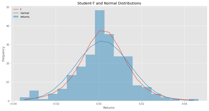
Here is how the normal and student-t PDF looks like for MSFT returns in the period we test.
ax = rets.returns.plot(kind='hist', bins=19, figsize=(14,7), density=True, alpha=0.5,
                       color=list(matplotlib.rcParams['axes.prop_cycle'])[1]['color'])

student_t_pdf = df.loc[df['dist'] == 't'].pdf.values[0]
pd.Series(student_t_pdf, x).plot(ax=ax, label='t')
normal_pdf = df.loc[df['dist'] == 'norm'].pdf.values[0]
pd.Series(normal_pdf, x).plot(ax=ax, label='normal')

ax.set_title(u'Student-T and Normal Distributions')
ax.set_xlabel(u'Returns')
ax.set_ylabel('Frequency')
plt.legend(loc="upper left")
ax.plot()
Back to our question now. How confident are we that tomorrow the price will not drop below 2% (-0.02)?
norm_cdf = np.cumsum(normal_pdf)
t_cdf = np.cumsum(student_t_pdf)
fig, (ax1, ax2) = plt.subplots(1, 2, figsize=(14,7))
fig.suptitle('CDF for Normal and T dists')
ax1.plot(x, norm_cdf)
ax2.plot(x, t_cdf)
plt.show()
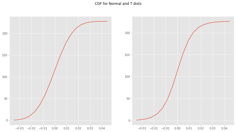
norm_cdf[np.where(x <= -0.02)][-1]
9.876651890962592
t_cdf[np.where(x <= -0.02)][-1]
8.086428763077489
According to the normal distribution, there is 9.9% probability that the price will drop below 2% while only 8.1% student-t probability. Someone, based on their risk tolerance, would be more confident to place some more money knowing that the estimate is much closer to the reality (well, historical reality)!
But, again, it is really up to us to use any distribution we feel comfortable with, based on the data we have, our risk level, and of course (when it comes to statistics) the tools to do our analysis easier.

